Spatial Joins Extended
Robin Lovelace, Jakub Nowosad, Jannes Muenchow
2026-01-28
Source:vignettes/join.Rmd
join.RmdThis vignette provides some further detail on the Vector attribute joining section (see https://geocompr.robinlovelace.net/attr.html#vector-attribute-joining ) of the Geocomputation with R book.
This vignette requires the following packages to be installed and attached:
We will use an sf object north_america with
country codes (iso_a2), names and geometries, as well as a
data.frame object wb_north_america containing
information about urban population and unemployment for three countries.
Note that north_america contains data about Canada,
Greenland and the United States but the World Bank dataset
(wb_north_america) contains information about Canada,
Mexico and the United States:
north_america = world %>%
  filter(subregion == "Northern America") %>%
  dplyr::select(iso_a2, name_long)
north_america
## Simple feature collection with 3 features and 2 fields
## Geometry type: MULTIPOLYGON
## Dimension: XY
## Bounding box: xmin: -171.7911 ymin: 18.91619 xmax: -12.20855 ymax: 83.64513
## Geodetic CRS: WGS 84
## # A tibble: 3 × 3
## iso_a2 name_long geom
## <chr> <chr> <MULTIPOLYGON [°]>
## 1 CA Canada (((-132.71 54.04001, -133.18 54.16998, -133.2397 53.8510…
## 2 US United States (((-171.7317 63.78252, -171.7911 63.40585, -171.5531 63.…
## 3 GL Greenland (((-46.76379 82.62796, -46.9007 82.19979, -44.523 81.660…
wb_north_america = worldbank_df %>%
  filter(name %in% c("Canada", "Mexico", "United States")) %>%
  dplyr::select(name, iso_a2, urban_pop, unemploy = unemployment)
wb_north_america
## # A tibble: 3 × 4
## name iso_a2 urban_pop unemploy
## <chr> <chr> <dbl> <dbl>
## 1 Canada CA 29014612 6.91
## 2 Mexico MX 98099040 4.81
## 3 United States US 259460378 6.17We will use a left join to combine the two datasets. Left joins are
the most commonly used operation for adding attributes to spatial data,
as they return all observations from the left object
(north_america) and the matched observations from the right
object (wb_north_america) in new columns. Rows in the left
object without matches in the right (Greenland in this
case) result in NA values.
To join two objects we need to specify a key. This is a variable (or
a set of variables) that uniquely identifies each observation (row). The
by argument of dplyr’s join functions lets
you identify the key variable. In simple cases, a single, unique
variable exist in both objects like the iso_a2 column in
our example (you may need to rename columns with identifying information
for this to work):
## Simple feature collection with 3 features and 5 fields
## Geometry type: MULTIPOLYGON
## Dimension:     XY
## Bounding box:  xmin: -171.7911 ymin: 18.91619 xmax: -12.20855 ymax: 83.64513
## Geodetic CRS:  WGS 84
## # A tibble: 3 × 6
##   iso_a2 name_long                                 geom name  urban_pop unemploy
##   <chr>  <chr>                       <MULTIPOLYGON [°]> <chr>     <dbl>    <dbl>
## 1 CA     Canada        (((-132.71 54.04001, -133.18 54… Cana…  29014612     6.91
## 2 US     United States (((-171.7317 63.78252, -171.791… Unit… 259460378     6.17
## 3 GL     Greenland     (((-46.76379 82.62796, -46.9007… NA           NA    NA
This has created a spatial dataset with the new variables added. The utility of this is shown in the figure below, which shows the unemployment rate (a World Bank variable) across the countries of North America.
## ## ── tmap v3 code detected ───────────────────────────────────────────────────────## [v3->v4] `tm_tm_polygons()`: migrate the argument(s) related to the scale of
## the visual variable `fill` namely 'breaks' to fill.scale = tm_scale(<HERE>).
## [v3->v4] `tm_polygons()`: migrate the argument(s) related to the legend of the
## visual variable `fill` namely 'title' to 'fill.legend = tm_legend(<HERE>)'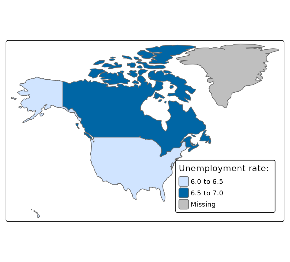
Figure 1. The unemployment rate (taken from World Bank statistics) in Canada and the United States to illustrate the utility of joining attribute data on to spatial datasets.
It is also possible to join objects by different variables. Both of
the datasets have variables with names of countries, but they are named
differently. The north_america has a name_long
column and the wb_north_america has a name
column. In these cases a named vector, such as
c("name_long" = "name"), can specify the connection:
## Simple feature collection with 3 features and 5 fields
## Geometry type: MULTIPOLYGON
## Dimension:     XY
## Bounding box:  xmin: -171.7911 ymin: 18.91619 xmax: -12.20855 ymax: 83.64513
## Geodetic CRS:  WGS 84
## # A tibble: 3 × 6
##   iso_a2.x name_long                            geom iso_a2.y urban_pop unemploy
##   <chr>    <chr>                  <MULTIPOLYGON [°]> <chr>        <dbl>    <dbl>
## 1 CA       Canada        (((-132.71 54.04001, -133.… CA        29014612     6.91
## 2 US       United States (((-171.7317 63.78252, -17… US       259460378     6.17
## 3 GL       Greenland     (((-46.76379 82.62796, -46… NA              NA    NA
Note that the result contains two duplicated variables -
iso_a2.x and iso_a2.y because both
x and y objects have the column
iso_a2. This can be solved by specifying all the keys:
left_join3 = north_america %>%
  left_join(wb_north_america, by = c("iso_a2", "name_long" = "name"))
left_join3
## Simple feature collection with 3 features and 4 fields
## Geometry type: MULTIPOLYGON
## Dimension: XY
## Bounding box: xmin: -171.7911 ymin: 18.91619 xmax: -12.20855 ymax: 83.64513
## Geodetic CRS: WGS 84
## # A tibble: 3 × 5
## iso_a2 name_long geom urban_pop unemploy
## <chr> <chr> <MULTIPOLYGON [°]> <dbl> <dbl>
## 1 CA Canada (((-132.71 54.04001, -133.18 54.16998… 29014612 6.91
## 2 US United States (((-171.7317 63.78252, -171.7911 63.4… 259460378 6.17
## 3 GL Greenland (((-46.76379 82.62796, -46.9007 82.19… NA NAJoins also work when a data frame is the first argument. However, for
them to work we need to drop the sf class.
left_join4 = wb_north_america %>%
  left_join(st_drop_geometry(north_america), by = c("iso_a2"))
left_join4
## # A tibble: 3 × 5
## name iso_a2 urban_pop unemploy name_long
## <chr> <chr> <dbl> <dbl> <chr>
## 1 Canada CA 29014612 6.91 Canada
## 2 Mexico MX 98099040 4.81 NA
## 3 United States US 259460378 6.17 United States
class(left_join4)## [1] "tbl_df" "tbl" "data.frame"In contrast to left_join(), inner_join()
keeps only observations from the left object
(north_america) where there are matching observations in
the right object (wb_north_america). All columns from the
left and right object are still kept:
inner_join1 = north_america %>%
  inner_join(wb_north_america, by = c("iso_a2", "name_long" = "name"))
inner_join1
## Simple feature collection with 2 features and 4 fields
## Geometry type: MULTIPOLYGON
## Dimension: XY
## Bounding box: xmin: -171.7911 ymin: 18.91619 xmax: -52.6481 ymax: 83.23324
## Geodetic CRS: WGS 84
## # A tibble: 2 × 5
## iso_a2 name_long geom urban_pop unemploy
## <chr> <chr> <MULTIPOLYGON [°]> <dbl> <dbl>
## 1 CA Canada (((-132.71 54.04001, -133.18 54.16998… 29014612 6.91
## 2 US United States (((-171.7317 63.78252, -171.7911 63.4… 259460378 6.17