Desire Lines Extended

This vignette builds on the transport chapter of the Geocomputation with R book by showing how to create multi-stage desire lines, from the ground-up.

It depends on these packages and datasets:

library(sf)
library(stplanr)
library(dplyr)
library(spDataLarge)
desire_lines = od2line(bristol_od, bristol_zones)
desire_rail = top_n(desire_lines, n = 3, wt = train)

The first stage is to create matrices of coordinates that will subsequently be used to create matrices representing each leg:

mat_orig = as.matrix(line2df(desire_rail)[c("fx", "fy")])
mat_dest = as.matrix(line2df(desire_rail)[c("tx", "ty")])
mat_rail = st_coordinates(bristol_stations)

The outputs are three matrices representing the starting points of the trips, their destinations and possible intermediary points at public transport nodes (named orig, dest and rail respectively). But how to identify which intermediary points to use for each desire line? The knn() function from the nabor package (which is used internally by stplanr so it should already be installed) solves this problem by finding k nearest neighbors between two sets of coordinates. By setting the k parameter, one can define how many nearest neighbors should be returned. Of course, k cannot exceed the number of observations in the input (here: mat_rail). We are interested in just one nearest neighbor, namely, the closest railway station:

knn_orig = nabor::knn(mat_rail, query = mat_orig, k = 1)$nn.idx
knn_dest = nabor::knn(mat_rail, query = mat_dest, k = 1)$nn.idx

This results not in matrices of coordinates, but row indices that can subsequently be used to subset the mat_rail. It is worth taking a look at the results to ensure that the process has worked properly, and to explain what has happened:

as.numeric(knn_orig)

## [1] 33 11 39

as.numeric(knn_dest)

## [1] 7 7 7

The output demonstrates that each object contains three whole numbers (the number of rows in desire_rail) representing the rail station closest to the origin and destination of each desire line. Note that while each ‘origin station’ is different, the destination (station 30) is the same for all desire lines. This is to be expected because rail travel in cities tends to converge on a single large station (in this case Bristol Temple Meads). The indices can now be used to create matrices representing the rail station of origin and destination:

mat_rail_o = mat_rail[knn_orig, ]
mat_rail_d = mat_rail[knn_dest, ]

The final stage is to convert these matrices into meaningful geographic objects, in this case simple feature ‘multilinestrings’ that capture the fact that each stage is a separate line, but part of the same overall trip:

mats2line = function(mat1, mat2) {
  lapply(1:nrow(mat1), function(i) {
    rbind(mat1[i, ], mat2[i, ]) %>%
    st_linestring()
  }) %>% st_sfc()
}
desire_rail$leg_orig = mats2line(mat_orig, mat_rail_o)
desire_rail$leg_rail = mats2line(mat_rail_o, mat_rail_d)
desire_rail$leg_dest = mats2line(mat_rail_d, mat_dest)

The results are visualised below:

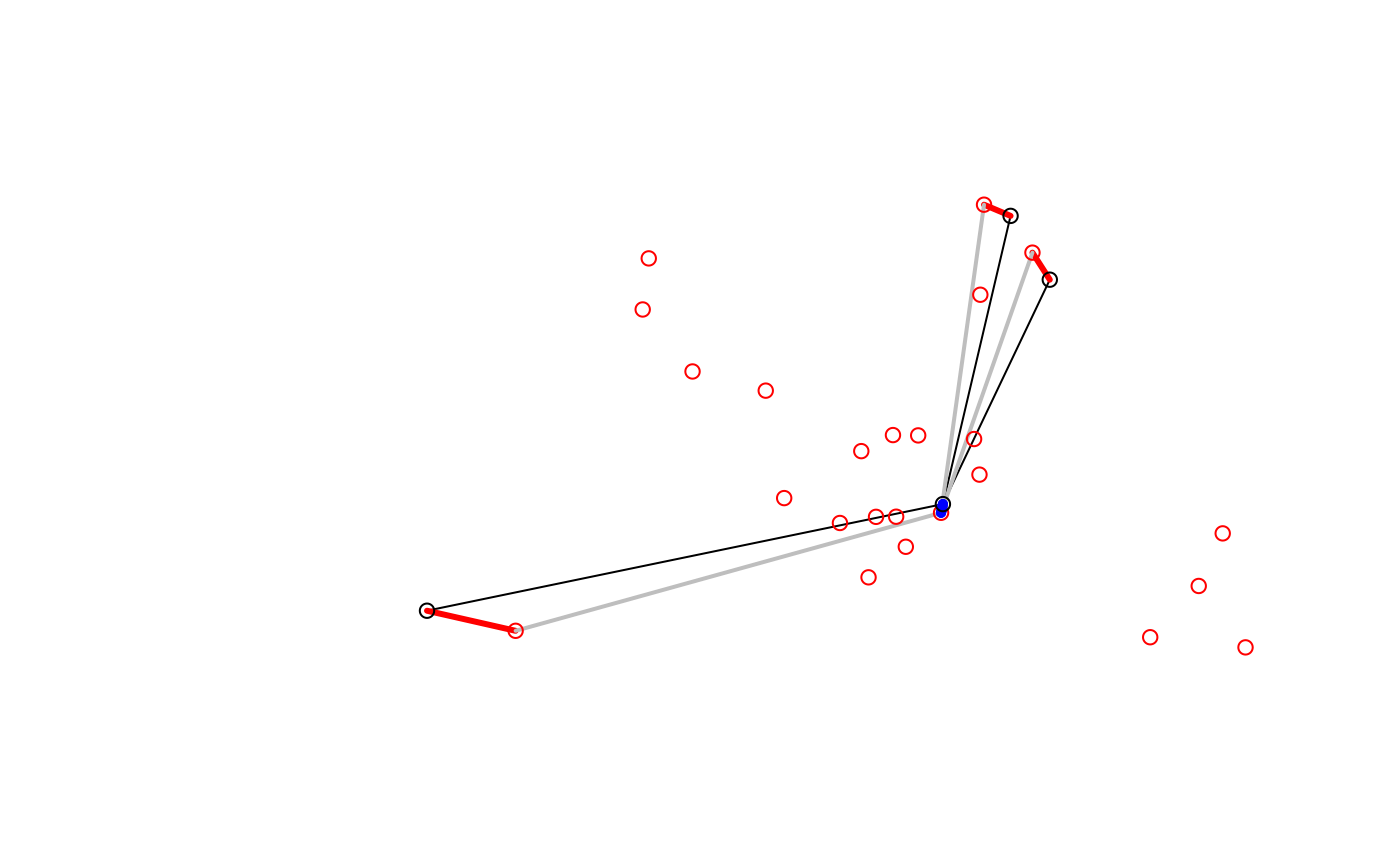
Station nodes (red dots) used as intermediary points that convert straight desire lines with high rail usage (black) into three legs: to the origin station (red) via public transport (grey) and to the destination (a very short blue line).

Desire Lines Extended

Robin Lovelace, Jakub Nowosad, Jannes Muenchow

2023-12-14